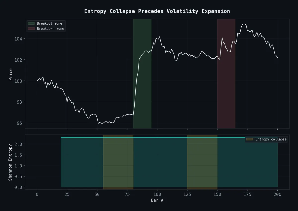
Entropy Collapse as a Volatility Timing Signal

The Verdict

ECVT is dead. I’m writing the headstone.

+198 bps on EURUSD hourly over two years. Gorgeous, right? Then -64 on EURGBP, -108 on GBPUSD, -88 on SPY, -17 on tick data. We even tried combining it with Hurst exponents — that made it worse. A signal that only works on one pair at one timeframe isn’t an edge. It’s a coincidence that survived long enough to get a backtest.

What follows is the full post-mortem. The information theory behind it is genuinely beautiful — Shannon entropy applied to return distributions to detect the coiling before a breakout. The math deserved better than what the market gave it. But the market doesn’t grade on elegance.

The Idea

Every volatility indicator you’ve ever used is a rearview mirror. ATR spikes after the breakout. Bollinger Bands expand after the range breaks. By the time you measure high volatility, you’ve already missed the entry.

We wanted to catch the coil before the spring.

Shannon entropy measures disorder. The intuition is almost too clean: before a breakout, price compresses. Returns cluster into a narrow range. The distribution tightens. Entropy drops. Then everything snaps.

The inspiration came from Singha (2025), “Hidden Order in Trades Predicts the Size of Price Moves” — tick-level Markov transition entropy predicting move magnitude with a 2.89× multiplier. We adapted it to hourly OHLC on forex. In retrospect, “adapted” is generous. We took a microscope-grade signal and squinted at it through binoculars. The granularity that made the original work was exactly what we threw away.

The Math

Shannon entropy for a discrete probability distribution:

H(X) = -Σ p(xᵢ) log₂ p(xᵢ) for i = 1 to n

Discretize a rolling window of returns into histogram bins. When returns concentrate (pre-breakout compression), fewer bins carry mass, entropy drops. When returns scatter (normal regime), entropy stays high.

Z-score normalization catches relative collapse — not absolute low entropy, but entropy significantly below its own recent mean. Different regimes have different baselines, so you need this.

Signal fires when the z-score drops below threshold: the distribution has compressed abnormally. Something is coiling.

This is sound information theory. The math never lied. The lie was assuming that every coil releases in a tradeable direction — turns out only EURUSD hourly ones do, apparently, and even that’s probably luck.

Implementation

The code works fine. The signal it produces doesn’t generalize. Here it is anyway, because the implementation isn’t what failed.

import numpy as np
import pandas as pd

def compute_shannon_entropy(returns: pd.Series, bins: int = 10) -> float:
    counts, _ = np.histogram(returns.dropna(), bins=bins)
    probs = counts / counts.sum()
    probs = probs[probs > 0]
    return -np.sum(probs * np.log2(probs))

def entropy_collapse_signal(df, lookback=50, bins=10, threshold=1.8):
    df = df.copy()
    df['returns'] = df['close'].pct_change()
    df['entropy'] = df['returns'].rolling(lookback).apply(
        lambda x: compute_shannon_entropy(x, bins=bins), raw=False
    )
    df['entropy_z'] = (
        (df['entropy'] - df['entropy'].rolling(200).mean())
        / df['entropy'].rolling(200).std()
    )
    df['signal'] = (df['entropy_z'] < -threshold).astype(int)
    return df

Direction from 20-period EMA slope. Entry at next bar open. 15-pip stop, 50-pip target, 24-bar timeout.

Results: EURUSD Hourly

44 trades over 2 years (Jan 2024 – Feb 2026).

Metric	Value
Trades	44
Win Rate	41%
Profit Factor	1.44
Total	+198 bps
Avg Win / Avg Loss	2.08×

Walk-forward: 10 out of 20 windows profitable. Aggregate OOS: +220 bps.

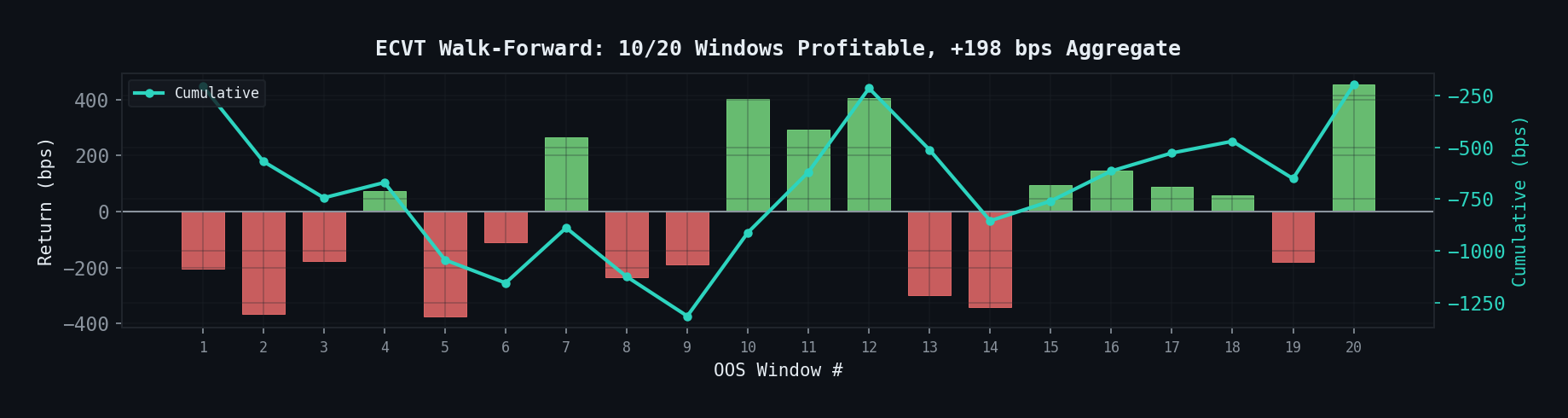Walk-forward equity curve Per-window OOS returns. 10/20 profitable — literally a coin flip.

In isolation, this looked like a marginal edge. PF 1.44 on 44 trades has roughly a 30% chance of showing up by pure chance. The 50% walk-forward hit rate is exactly what a random signal produces. But we wanted to believe the information theory — the math was so clean — so we kept testing. That’s the trap. Beautiful theory makes you generous with ambiguous data.

The Kills

EURGBP Hourly

If entropy collapse is structural to forex, it should transfer to correlated pairs. We tested on EURGBP — 28.8M ticks from Darwinex, aggregated to 12,801 hourly bars. Same parameters.

Metric	EURUSD	EURGBP
Trades	44	23
Win Rate	41%	30%
Profit Factor	1.44	0.76
Total	+198 bps	-64 bps
Stop-outs	—	61%

Dead on arrival. Only 16 OOS trades across 9 walk-forward windows. That’s not a small sample — it’s a rounding error.

GBPUSD Hourly

-108 bps. The entropy signal walked into a different microstructure and bled out.

Equities (SPY, QQQ, IWM, GLD, TLT)

SPY: 9 trades, -88 bps, 89% stop-outs. The others fired 0–5 times over two years. Not enough to evaluate, and that is the evaluation. Session-based markets don’t have continuous entropy dynamics — they close at 4pm and gap at 9:30am. The signal doesn’t underperform on equities. It barely exists there.

Tick Data

We went back to the source. If OHLC was too coarse, maybe tick-level data would recover the Singha result. -17 bps. The hourly aggregation wasn’t hiding a tick-level edge — it was manufacturing one through information loss. The artifact lived in the compression, not in the market. That one hurt. We’d been trading a lossy-encoding glitch.

ECVT + Hurst Exponent

Hurst measures persistence. Below 0.5 = mean-reverting, above 0.5 = trending. Combining with ECVT seemed logical: entropy collapse says something is about to happen, Hurst says what kind of regime you’re in.

-86 bps OOS. Worse than either signal alone. Two marginal signals don’t compound into an edge. They compound into more noise wearing a fancier hat.

Summary of Death

Test	Result
EURUSD 1H	+198 bps
EURGBP 1H	-64 bps
GBPUSD 1H	-108 bps
SPY daily	-88 bps (9 trades)
EURUSD ticks	-17 bps
ECVT + Hurst OOS	-86 bps
Everything except EURUSD 1H	Dead

One green row. Five red ones. The green one has 44 trades and a coin-flip walk-forward. The prosecution rests.

Why the Math Was Right and the Strategy Was Wrong

The entropy collapse pattern is real. I’ve seen it with my own eyes in every consolidation-before-breakout sequence. Returns compress, entropy drops, range breaks. Observable, repeatable, grounded in solid information theory.

Three things killed it:

Compression doesn’t pick a direction. Entropy collapse says magnitude is coming. It says nothing about which way. We bolted on an EMA-slope heuristic for direction, and it worked on EURUSD and failed everywhere else. Singha’s paper explicitly predicted magnitude, not direction. We grafted on directionality and the graft rejected.

OHLC is a lobotomy. Singha used tick-level Markov transition matrices. We used histogram bins on hourly returns. The information content gap between those two representations is enormous. Our adaptation was a summary of a summary. Like trying to diagnose a patient from a photograph of their medical chart.

44 trades is not a sample. You need 200+ to separate PF 1.44 from luck with any real confidence. We had 44 on the one pair that worked and fewer everywhere else. A single outlier trade swings the PF by 0.3 in a sample that small. We weren’t measuring an edge. We were measuring weather.

What “Dead” Means

A strategy that works on one asset at one timeframe is not a strategy. It’s a coincidence that happened to land inside a backtest window.

ECVT is asset-specific (EURUSD only) AND timeframe-specific (hourly OHLC only). It dies on other pairs, dies on equities, dies on tick data, and gets worse when you add complementary signals. Every generalization axis came back red. We can’t explain why EURUSD hourly entropy collapses would be tradeable but EURGBP ones wouldn’t — because they probably aren’t. The EURUSD result is noise that looks like a pattern.

The formal kill criteria: if you can’t identify why it works on one instrument and not others, and you can’t reproduce the edge on related instruments, you’re curve-fitting to noise. We couldn’t. So we stopped.

Status: Dead. The underlying observation — that entropy of returns drops before large moves — remains a legitimate insight about market microstructure. But “legitimate insight” and “tradeable edge” are separated by an ocean, and we sank halfway across.

The entropy collapse pattern deserves better methodology than ours. Tick-level Markov transitions on a broader universe, maybe. But this implementation, with these parameters, on OHLC data? Buried.

Headstone reads: “Looked promising on one pair. Died on contact with everything else. 2024-2026.”

Code: quant-research. See 31 Strategies Tested for where this fits in the larger picture.