From PyTorch to 27 Megabytes: A Neural Net Trade Filter on a Budget VPS

Update (March 2026): The NN filter got pulled from live trading around February 25, 2026. It was overfitting on 302 trades. The raw strategy without it proved purer. Full autopsy below.

40% of Your Trades Lose. Can a Neural Net Fix That?

Our EURUSD 30-minute strategy survived five rounds of honest deflation. The floor: 302 trades, 59.6% win rate, +463 pips, profit factor 1.48 over 2.5 years.

That means 121 trades hit stop-loss. Some of them felt wrong before entry — Monday morning chop, mid-session noise, stale setups lingering past their expiry date. Surely a neural network could learn which ones to skip?

No. But we learned things worth keeping on the way to that answer.

The Patterns Are Real. The Training Set Isn’t.

Before training anything, we ran post-hoc analytics on the 302 trades:

Monday alone carries 80% of total profit (PF 3.56, 73.9% WR). Tuesday and Thursday bleed. This held for 2.5 years.

Same story intraday: 09:00 UTC (London open) and 13:00 UTC (NY open) print money. Mid-session hours give it back. The edge clusters at session transitions.

These patterns are real. A human could just trade Mondays and session opens with hard rules. But we wanted soft boundaries — probabilistic filters, nuance, the sophistication that makes you feel smart. That sophistication needed orders of magnitude more data than we had.

We had a spreadsheet. We reached for deep learning.

Eleven Features, Zero Price Data

The NN never sees price. The strategy already made its structural decision. The network only sees metadata about the setup:

features = [
    is_london_open,          # session (binary)
    is_long,                 # direction (binary)
    hour_sin, hour_cos,      # cyclical hour encoding
    dow_sin, dow_cos,        # cyclical day-of-week encoding
    signal_age_normalized,   # how stale is this setup (0-20 days)
    signal_size_normalized,  # setup size in pips
    risk_pips_normalized,    # SL distance
    is_monday,               # Monday flag
    is_session_open,         # session-open hour flag
]

Cyclical encoding matters. Hour 23 and hour 0 are neighbors, not 23 apart. Without it, the network thinks Friday is as far from Monday as possible.

Deliberately Tiny. Still Too Big.

Input (11) → Linear(32) → ReLU → Linear(16) → ReLU → Linear(1) → Sigmoid

Three layers. 593 parameters. We made it small on purpose — 302 trades is tiny, a deeper network would memorize everything.

It memorized everything anyway.

Training: ensemble of 10 models with different random seeds, state dicts averaged. BCEWithLogitsLoss, Adam, 300 epochs, batch 32. The ensemble was supposed to smooth out seed-dependent noise. With 302 samples, it smoothed noise into a different flavor of noise.

The In-Sample Mirage

EURUSD at threshold P(win) ≥ 0.45:

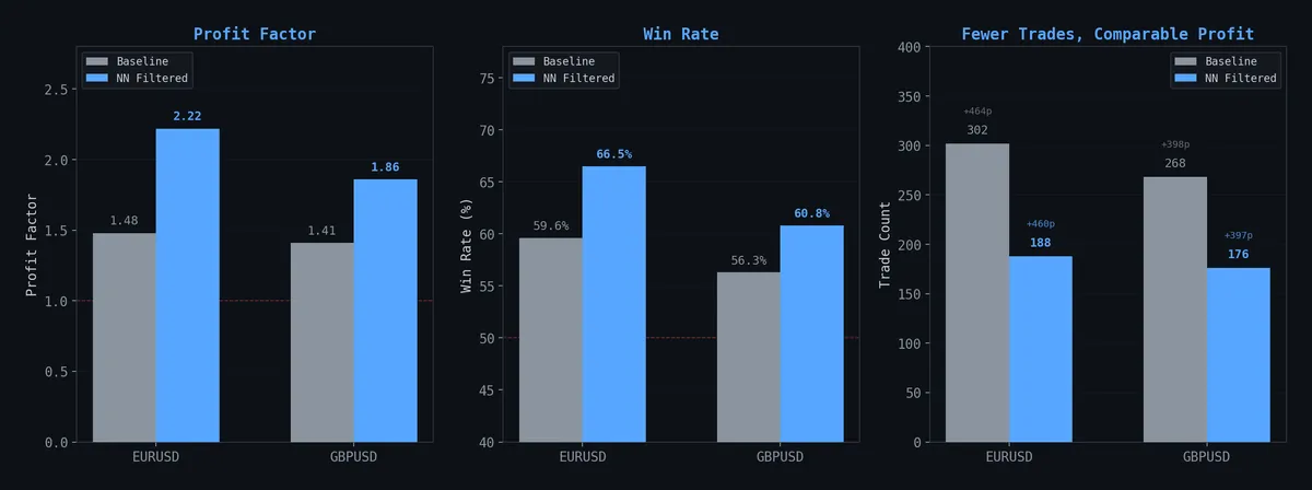
Metric	Baseline	NN Filtered	Change
Trades	302	188	-38%
Win Rate	59.6%	66.5%	+6.9pp
Profit Factor	1.48	2.22	+50%
Total Pips	+463	+460	-0.6%

Same profit, 38% fewer trades, dramatically better profit factor. On paper, the network surgically removed noise without sacrificing edge. Beautiful.

The equity curve looked cleaner:

Filtered (blue) tracks the same endpoint as baseline (gray) with less drawdown and fewer flat stretches. The kind of chart that makes you want to ship immediately.

That feeling? That’s the feeling right before you overfit.

The Score Distributions

The P(win) scores weren’t perfectly separated — 58.6% OOS accuracy. Wins clustered slightly higher, losses slightly lower. The 0.45 threshold cut the left tail where losses dominate.

58.6% OOS accuracy on binary classification with 302 samples. That’s barely above a coin flip. “Barely above chance on a small sample” and “noise” are the same thing. We should have stopped here.

Threshold Tuning on Static

We chose 0.45 because it sat at the knee: PF plateaued at ~2.2, total pips still tracked baseline. Above 0.50, the filter killed real winners. Below 0.40, marginal trades survived.

We were fitting a curve to static. But the chart looked convincing, so we kept going.

Cross-Pair: Dead on Arrival

Tested the EURUSD model on GBPUSD. Transfer accuracy: 44%. Worse than flipping a coin. Temporal patterns are pair-specific — Monday dominance on EURUSD says nothing about GBPUSD.

A standalone GBPUSD model showed the same in-sample trick — PF jumping from 1.41 to 1.86 while preserving pips. Same 302-sample mirage, different accent.

EURGBP baseline PF was 1.08. We didn’t even bother filtering a corpse.

The Baseline Strategy Is Real (The NN Isn’t)

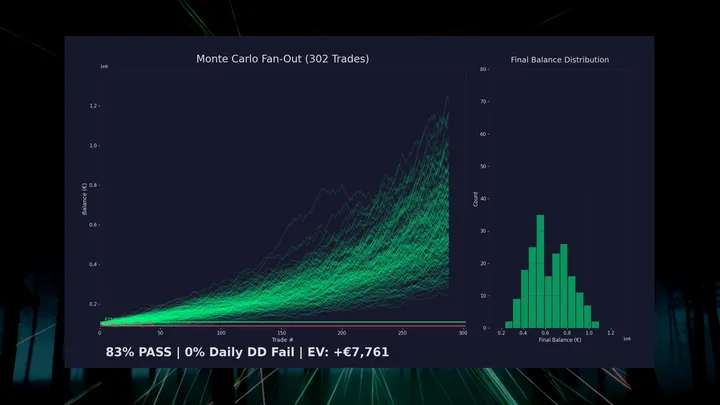
Monte Carlo bootstrap — 200 simulated equity paths:

Even the 5th percentile path produces +188 pips. Monthly breakdown:

21 of 32 months profitable. Worst: -38 pips. Best: +129 pips.

Max drawdown: -101 pips (~12% account drawdown at 1% risk).

These stats validate the baseline strategy. The gap-fill physics, the deflation layers, the tick validation — that’s where the edge lives. The Monte Carlo proves the underlying trade distribution holds up.

The NN’s contribution? Unvalidated on any time period that matters.

The VPS Problem (This Part Actually Worked)

Live trading runs on a $9/month Contabo Windows VPS — 2 vCPUs, 4GB RAM, MT5, Task Scheduler firing every 30 minutes.

PyTorch CPU-only: ~2GB installed. On a 4GB VPS already running MT5 and Windows, that’s a death sentence. But our model is 593 parameters. Three matrix multiplications and two ReLUs. We don’t need automatic differentiation. We need multiplication.

PyTorch → Numpy: 2GB to 3.7KB

This engineering holds up regardless of whether the NN was any good.

# Export once (requires torch, run locally):
def export_weights(pt_path, json_path):
    checkpoint = torch.load(pt_path, map_location="cpu")
    sd = checkpoint["model_state_dict"]
    weights = {
        "W1": sd["net.0.weight"].tolist(),
        "b1": sd["net.0.bias"].tolist(),
        # ... same for layers 2, 3
    }
    Path(json_path).write_text(json.dumps({"weights": weights, ...}))

# Inference (numpy only, runs on VPS):
class TradeScorer:
    def _forward(self, x: np.ndarray) -> np.ndarray:
        h1 = np.maximum(0, x @ self._W1.T + self._b1)   # ReLU
        h2 = np.maximum(0, h1 @ self._W2.T + self._b2)  # ReLU
        return (h2 @ self._W3.T + self._b3).squeeze(-1)  # logit

Weight files: 21KB JSON. Runtime memory: 3.7KB. Inference: ~0.1ms per trade. The VPS went from “can’t install torch” to “doesn’t need torch.”

If you ever need to deploy a small PyTorch model to a resource-constrained environment, this is the move. Export weights as JSON, reconstruct the forward pass in numpy. No ONNX, no TorchScript, no runtime baggage. Just matrix math.

Belt and Suspenders

Two-layer defense architecture:

1. Signal engine: .filter() hard-drops orders with P(win) < threshold
2. Trade orchestrator: defensive gate catches anything that slips through

This defense-in-depth pattern for trade execution is sound engineering regardless of what model sits behind it.

The Ghost Bars

This was the real discovery. Not the NN. Not the filter. This.

While deploying, we switched from a third-party data API to MT5’s native copy_rates_from_pos(). Same symbol, same timeframe, same bar count. Different results.

The API was returning bars into Saturday — synthetic weekend data that doesn’t exist in the real market. These phantom bars ate slots in our 500-bar window, pushing out real trading days:

Source	500 bars span	Last bar
Third-party API	Feb 11 → Feb 21 (Sat)	Saturday 17:00 ⚠️
MT5 direct	Feb 6 → Feb 20 (Fri)	Friday 23:30 ✅

MT5 gives 5 extra real trading days of history. Two pending signals that existed under the API vanished under MT5 — correctly identified as already invalidated by price action the API’s truncated window couldn’t see.

Your data provider is part of your strategy. Same logic, different data, different trades. If you’re feeding MT5 from a third-party API, compare its output against MT5’s native data. Differences aren’t edge cases — they’re execution divergence. We cut out the middleman.

Week 1 Live: Three Trades, No NN

Deployed February 17, 2026 with €10,000 demo. Pure baseline, no filter:

#	Date	Direction	Result	Pips	Net P&L
1	Feb 18	LONG	❌ SL	-10.0	-€181
2	Feb 19	LONG	✅ TP	+10.7	+€229
3	Feb 20	LONG	❌ SL	-8.5	-€193

Week 1: -€145.67 (-1.46%). One win, two losses. Three trades is noise, not signal. You can’t draw a line through three points and call it a trend.

The Epilogue: We Overfitted

The original post ended asking: “does the filter’s edge persist live, or did we overfit 302 trades?”

We overfitted 302 trades.

Around February 25, the NN filter got pulled from the live VPS. The math is simple: 302 training samples isn’t enough for a neural network to learn generalizable patterns, even one with only 593 parameters. The conditional patterns — Monday dominance, session-open clustering — are real features of EURUSD 30-minute price action. But a network trained on 302 examples of those patterns memorizes the specific 302 trades, not the underlying structure.

The raw IPDA CE strategy kept trading without the filter. As of early March, the account sat at €9,540.23, recovering from -6.14% max drawdown to -4.6%. The edge lives in the gap-fill physics and the deflation layers — the work we did before any ML touched it. The NN was decoration on a building that stands fine on its own.

GBPUSD never went live. The strategy is asset-specific. Transfer learning across forex pairs produced below-coin-flip accuracy, and the standalone GBPUSD model had the same small-sample disease.

What survived:

• The baseline strategy. Five deflation rounds, tick-validated, spread-adjusted. Still trading. Still profitable.
• The deployment engineering. PyTorch-to-numpy export, two-layer defense, VPS resource management. These patterns work for any small model.
• The ghost bar discovery. Data provider divergence is real and nobody talks about it enough.
• The instinct to ask “did we overfit?” That was the right question. The mistake was not waiting long enough for the answer.

What died:

• The NN filter. 302 samples, 593 parameters, 10-seed ensemble — none of it was enough. The backtest looked clean because the model learned the training set, not the market.
• Cross-pair dreams. GBPUSD needs its own validation pipeline, not a EURUSD hand-me-down.

The lesson is ancient: if your training set fits in a spreadsheet, you don’t need a neural network. Hard rules — trade Mondays, skip mid-session — would have captured the same patterns without the overfitting risk. We reached for ML because it felt sophisticated. The market doesn’t reward sophistication. It rewards being right.

What’s Next

• Raw strategy continues — IPDA CE on EURUSD 30m, no filter, no decorations
• Weekly equity updates — real performance, no cherry-picking. The account is underwater but climbing back.
• Hard rules over soft models — if conditional patterns persist with enough forward data, we’ll use day/hour filters. Not neural networks trained on 302 trades.

---

Part of an ongoing series documenting live systematic trading with honest outcomes. Previous: Starting from the End: Prop Firm Challenges as Variance Optimization.